Alain Le Bot - Portrait

Tribology and System Dynamics Laboratory - CNRS

Ecole Centrale de Lyon

36, avenue Guy de Collongue, 69134 Ecully, FRANCE

Phone: +33 4 72 18 62 75

Email: alain.le-bot@ec-lyon.fr

Statistical Energy Analysis (SEA)

High frequency in vibroacoustics

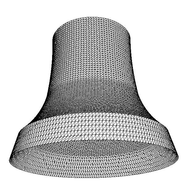
Classical methods in acoustics and structural dynamics are based on the resolution of the governing equation by finite element method. But the latter requires a fixed number of degrees of freedom per wavelength. And since the more the frequency increases, the more the wavelength decreases, the total number of degrees of freedom rapidly becomes huge.
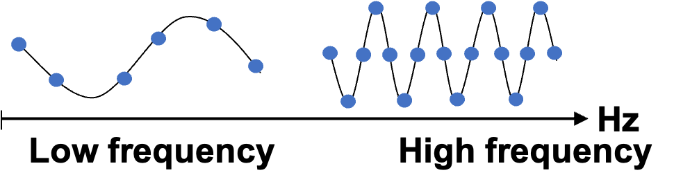
High frequency wavelength and degrees of freedom

The number of degrees-of-freedom per wavelength is fixed. At high frequency, the wavelength is short and the total number of degrees-of-freedom is large.
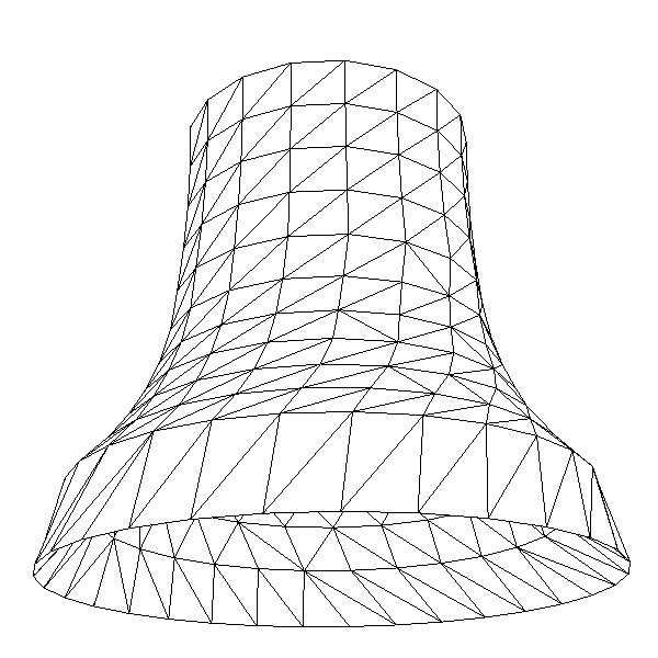
Mesh low frequency

Mesh of a Mersenne bell well suited for low frequencies.
Mesh high frequency

Mesh of a Mersenne bell well suited for high frequencies.

Due to limited capabilities of computers, finite element softwares cannot perform calculations up to the high frequency range.

structure car aircraft ship
frequency ~500 Hz ~50 Hz ~5 Hz
Maximal frequency by finite element method for a model of the order of million degrees of freedom.

The increase of frequency also induces an increase of the number of natural modes of structure. Rapidly, the population of modes becomes very large. Thus, the mathematical methods based on the development of solution on modal basis become intractable.

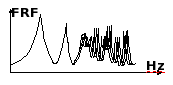
Numerical models require the knowledge of many parameters such as exact geometry, material properties, applied forces... But some of them are generally not well-known and we must consider that all input data have an uncertainty. However, results of computation become more sensitive to uncertainty when the frequency increases. So, even if we had very strong computers capable of doing calculations up to infinite frequency, those results would be not reliable.
Sensitivity of frequency response function

In high frequencies, the sensitivity is large. Frequency response functions of different calculations do not match.
The principles of statistical energy analysis (SEA)

SEA is a statistical theory of vibroacoustics [1, 2, 3]. This is a theory well suited to complex structures vibrating in the high frequency domain under random excitations. It is based on the application of concepts and methods of statistical physics to the study of energy exchange between acoustical and mechanical components. The pioneers of SEA were largely inspired by statistical physics and recent advances in SEA continue to be inspired by it. SEA is a demonstration that in engineering sciences, a conceptual revolution is still possible.

In statistical vibroacoustics, sources of vibration are assumed to be random, wideband, and uncorrelated. The ideal case is that of independent and identically distributed (i.i.d.) stationary white noise. In practice, we assume that the power spectral density of the sources is flat within a certain frequency band \([ \omega-\Delta\omega/2, \, \omega+\Delta\omega/2]\) and that the cross-power spectral densities are zero. The stochastic nature of sources is an essential ingredient for applying a statistical approach. Instead of predicting the full field of vibration at any point and any time, we focus on the probabilistic expectation of vibrational energy.

Modes are the sites where vibrational energy localizes. They play the same role in statistical vibroacoustics as molecules or atoms do in statistical physics. They are microscopic entities whose individual behavior remains unknown, yet which form a statistical population whose overall behavior is predictable. Their number is assumed to be large (large population of modes) and their frequency distribution follows the so-called Gaussian orthogonal ensemble (fully disorganized population of modes).

Since the sources are white noise, the vibrational energy carried by a given mode changes at every instant. Modes are therefore grouped to constitute subsystems. A subsystem is defined as a packet of similar modes in a structural component of the system. These can be rod, beam, plate, shell, acoustical cavity but, a subsystem can also be selected modes within a structural component like flexural modes in plate, longitudinal modes, or torsional modes in rods. Within a subsystem, modes are orthogonal. In particular, they do not exchange energy between them. They receive their vibrational energy directly from the random sources.

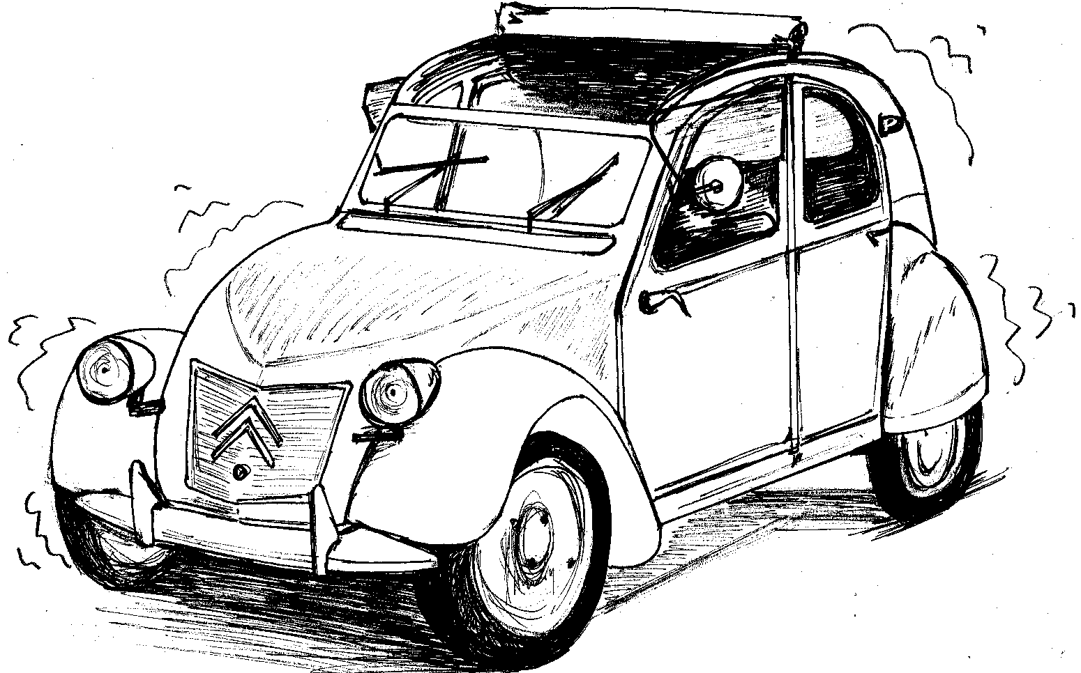
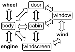
A structure is divided in n subsystems. The subsystems defined as group of orthogonal modes of the same structural component, may be coupled with subsystems of neighboor components. The couplings realize the path by which the vibrational energy flows throughout the entire structure. However, all couplings are assumed to be weak. This is an important condition to ensure that a thermalization state is reached by the entire system.

Example of complex structure

Example of complex structures whose components are weakly coupled

Set of subsystems

Set of subsystems to describe the complex structure.

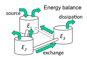
Subsystems behave like energy reservoirs containing a specific form of energy, acoustical or vibrational, longitudinal, transverse, flexural waves... These reservoirs can receive, dissipate, and exchange energy with their neighbours. So, the global situation is the following. In each susbsystem, modes receive in average the same amount of energy from the sources. This state of equipartition of energy is certainly the most important consequence of the assumptions of random sources, large and disorganized population, and weak couplings. Of course, at a fixed time, equipartition does not mean that all modes have exactly the same energy. But in average (probabilistic expectation or time-average by ergodicity), all modes have the same energy.

SEA is the theory which describes these exchanges of energy. SEA is like thermodynamics of acoustical and structural vibrations, confined within the audio frequency band, 20 Hz to 20 kHz, which is very low compared with thermal frequencies of usual thermodynamics.

SEA frequency spectrum compared to thermodynamics

SEA focuses on energy transfers of audio frequency band while thermodynamics applies to thermal frequencies.

Energy balance

Subsystems receive energy from external sources and neighbour subsystems, and lose energy either by internal damping or exchange with neighbour subsystems. In steady-state regime, the energy balance of subsystem i reads,

\[ P_{\mathrm{inj},i} + \sum_{j\neq i} P_{j \to i} = P_{\mathrm{diss},i} + \sum_{j\neq i} P_{i \to j} \]

where the gain appears on the left-hand side and the losses on the right-hand side. \(P_{\mathrm{inj},i}\) is the power supplied by external sources to susbsytem \(i\), \(P_{\mathrm{diss},i}\) the power being dissipated in subsystem \(i\) by internal damping, \(P_{j \to i}\) (respectively \(P_{i \to j}\)) the power supplied through couplings by subsystem \(j\) to \(i\) (respectively by \(i\) to \(j\)). In accordance with the steady-state assumption, no energy accumulation term appears.

The power dissipated in subsystem \(i\) is proportional to its vibrational energy \(E_i\). One introduces the so-called damping loss factor \(\eta_i\) such that,

\[ P_{\mathrm{diss},i} = \omega\eta_i E_i \]

where \(\omega\) is the central frequency (rad/s) of the souces.

When two subsystems \(i\) and \(j\) are physically connected, a part of the energy of \(i\) is transmitted to \(j\) and conversely. From the point of view of \(i\), the energy transmitted to \(j\) per unit time, or transmitted power noted \(P_{i \to j}\), is lost. We may therefore introduce the coupling loss factor \(\eta_{ij}\) such that the power lost by \(i\) through the coupling with \(j\) is

\[ P_{i \to j} = \eta_{ij} \omega E_i \]

This equation is similar to previous one for internal dissipation. It must also be considered that subsystem \(j\) can provide subsystem \(i\) with,

\[ P_{j \to i} = \eta_{ji} \omega E_j \]

Coupling loss factors \(\eta_{ij}\) and \(\eta_{ji}\) are not independent. They are linked by the reciprocity relationship,

\[ N_i \eta_{ij} = N_j \eta_{ji} \]

where \(N_i\) is the number of modes of subsystem \(i\). The exchanged power can then be written as the difference of modal energies.

\[ P_{ij} = P_{i \to j} - P_{j \to i} = \omega \eta_{ij} N_i \left( \frac{E_i}{N_i} - \frac{E_j}{N_j} \right) \]

and we see that the vibrational power exchanged by coupling is proportional to the difference of modal energies. Consequently, the energy flows from subsystem having a high modal energy to that with a low modal energy. This law, due to R.H. Lyon is the foundation of an analogy with Clausius' principle which states that heat flows from high to low temperatures.

By substituting the expressions of dissipated and exchanged powers into the power balance, one obtains a set of linear equations on the modal energies \(E_i/N_i\). We get,

\[ \omega \left( \begin{array}{cccc} N_1 \sum_j \eta_{1j} & -N_2 \eta_{21} & \dots & -N_n \eta_{n1} \\ -N_1 \eta_{12} & N_2 \sum_j \eta_{2j} & & -N_n \eta_{n2} \\ \vdots & & \ddots & \vdots \\ -N_1 \eta_{1n} & -N_2 \eta_{2n} & \dots & N_n \sum_j \eta_{nj} \end{array} \right) \left( \begin{array}{c} E_1 / N_1 \\ E_2 / N_2 \\ \vdots \\ E_n / N_n \end{array} \right) = \left( \begin{array}{c} P_{\mathrm{inj},1} \\ P_{\mathrm{inj},2} \\ \vdots \\ P_{\mathrm{inj},n} \end{array} \right) \]

This is a symmetric system that can be solved by any standard method.

All these considerations on energy in SEA can be summarized in the following figure,

Energy exchanges in SEA

Energy exchanges in SEA. Sub-systems behave like energy tanks. All tanks can receive, dissipate or exchange energy.

Entropy balance

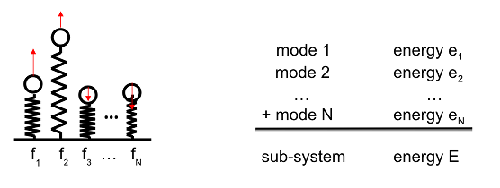
A SEA subsystem is a packet of \(N\) resonators with different natural frequencies \(f_1, \dots , f_N\). Each mode contains a vibrational energy \(e_k\) and the sum is \(E = \sum_k e_k\). But since sources are random, the distribution of the energy \(E\) over the \(N\) modes is fluctuating in time. The only quantity assumed to be known is the expectation of the sum of modal energies that we have noted \(E\).

Energy repartition over modes

The entropy associated to this dynamical system is a measure of the number of possibilities to share energy \(E\) over \(N\) modes. This is [4],

\[ S(E,N) = k_\text{B} N \left[ 1 + \log\left( \frac{2\pi E}{h \omega N} \right) \right] \]

where \(k_\text{B}\) is Boltzmann's constant and \(h\) is Planck's constant. This entropy is a state function which only depends on the extensive quantities vibrational energy \(E\) and number of modes \(N\). The vibrational temperature is defined as for any thermodynamical system by,

\[ \frac{1}{T} = \left( \frac{\partial S}{\partial E} \right)_N \]

One obtains,

\[ T = \frac{E}{k_\text{B}N} \]

The vibrational temperature is therefore equal to the modal energy divided by Boltzmann's constant.

The number of modes of a subsystem is constant. Only the vibrational energy can vary. The variation of entropy is therefore obtained by differentiating the expression of entropy thus, \(dS=dE/T\). In case of a single source of power \(P\), the energy supplied to subsystem during \(dt\) is \(dE=P dt\). The vibrational temperature being \(T=E/k_\text{B}N\), the rate of entropy created by the source is,

\[ \frac{dS_{\text{inj},i}}{dt} = k_\text{B} \frac{P_{\text{inj},i}N_i}{E_i} \]

This rate is positive since the source supplies energy to subsystem and therefore warms it.

In a similar way, the rate of entropy due to dissipation can be calculated. It yields,

\[ \frac{dS_{\text{dis},i}}{dt} = -k_\text{B} \omega \eta_i N_i \]

We can observe that this rate is negative. Dissipation processes therefore tend to decrease the entropy level. This is the converse of what happens in thermodynamics! This result can be explained by the fact that here, dissipation is responsible of a decrease of internal energy and therefore cool down the system. Indeed, this decrease must be accompanied by an increase of the thermodynamical entropy.

Finally, one can calculate the entropy rate created during the energy exchange between two adjacent sub-systems. It yields,

\[ \frac{dS_{ij}}{dt} = k_\text{B} \omega (\eta_{ij} E_i - \eta_{ji} E_j) \left( \frac{N_i}{E_i} - \frac{N_j}{E_j} \right) \]

It is always positive as it can be easily checked. This is the expression of the second principle of thermodynamics in the particular framework of SEA.

The global entropy balance is the following,

\[ \frac{dS}{dt} = \sum_{i=1}^N \left( \frac{dS_{\text{inj},i}}{dt} + \frac{dS_{\text{dis},i}}{dt} \right) + \sum_{i>j} \frac{dS_{ij}}{dt} = 0 \]

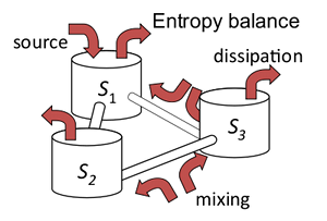
which is summarized in the following diagram,

Vibroacoustical entropy exchanges in SEA

Vibroacoustical entropy exchanges in SEA. All sub-systems behave like entropy tanks. These tanks can receive, dissipate and create entropy by mixing energy.

  1. A. Le Bot, Entropy in statistical energy analysis, Journal of the Acoustical Society of America, vol. 125, p. 1473-1478, 2009.

  2. A. Le Bot, A. Carcaterra, D. Mazuyer, Statistical vibroacoustics and entropy concept, Entropy, vol. 12, p. 2418-2435, 2010.

  3. A. Le Bot, Entropy in sound and vibration: towards a new paradigm, Proc. R. Soc. A, 473, 20160602, 2017.

Domain of validity

Like any physical theory, statistical energy analysis (SEA) has a domain of validity. SEA is a statistical theory derived from linear acoustics and structural wave equations. SEA relies fundamentally on the concept of the vibrational field being in a state of thermalization. To be more specific : the sources must be random, the vibrational field within each subsystem must be diffuse, and energy exchange between adjacent subsystems must be weak.

The sources must be random, centred, stationary, uncorrelated and broadband. Let \(f_i(t)\) be \(n\) random external forces applied to the system.

  • Centred: the expectations are zero \(\langle f_i(t) \rangle =0\).
  • Stationary: the cross-correlations \(R_{ij}(\tau)=\langle f_i(t) f_j(t+\tau) \rangle\) do not depend on \(t\).
  • Uncorrelated: the cross-correlations are zero \(R_{ij}(\tau)=0\) when \(i\neq j\)
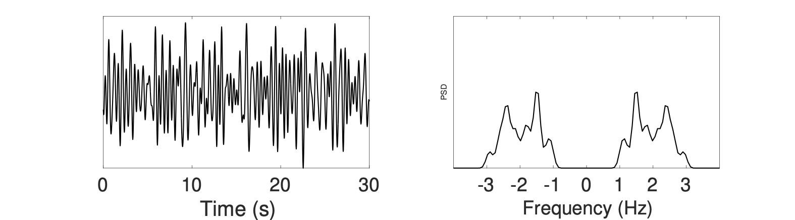
  • Broadband: the power spectral densities \(S_{ii}(\omega)\) are flat within a broad frequency band \([\omega_0-\Delta\omega, \, \omega_0+\Delta\omega]\).
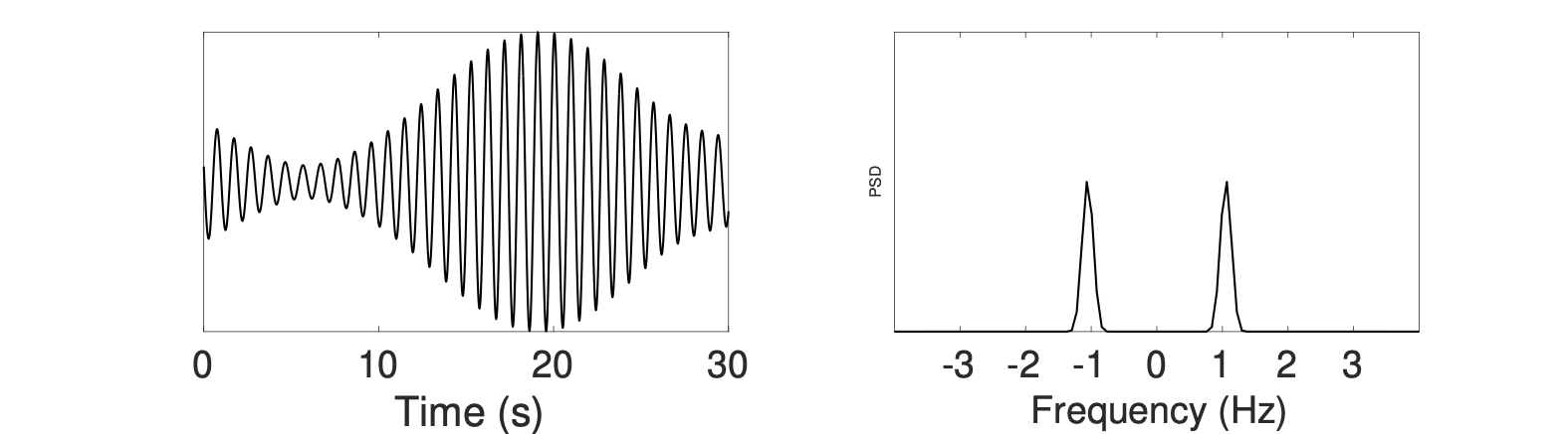
Narrow band noise

Example of narrow band noise. Not suited for SEA.

Broadband noise

Example of broadband noise. Well suited for SEA.

Wavefield in all subsystems must be diffuse. A diffuse field is a vibrational field for which the spatial distribution of energy is homogeneous and the directional distribution is isotropic.

Modes exhibit a shape defined by nodal lines—where energy is zero—and antinodes—where energy is at a maximum. By nature, a single mode cannot produce a diffuse field. However, a large number of modes with nodal lines and antinodes distributed randomly across the subsystem can generate a diffuse field. Consequently, the first condition is large number of modes \(N\).

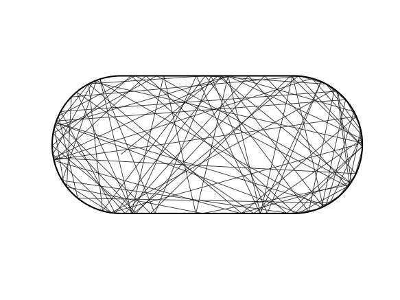
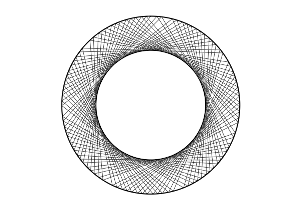
In geometrical acoustics, a vibration field consists of rays propagating at the group velocity and reflecting on the boundaries. Energy mixing—a prerequisite for the emergence of a diffuse field—therefore depends on ray dynamics. In the mathematical theory of billiards, it is well known that certain geometries are ergodic while others are not; the Bunimovitch stadium and Sinai billiard are ergodic, whereas the disk is not.

Ergodic billiard

Ray path in an ergodic billiard. Emergence of a diffuse field.

non-ergodic billiard

Ray path in a non-ergodic billiard. Strongly non homogeneous field.

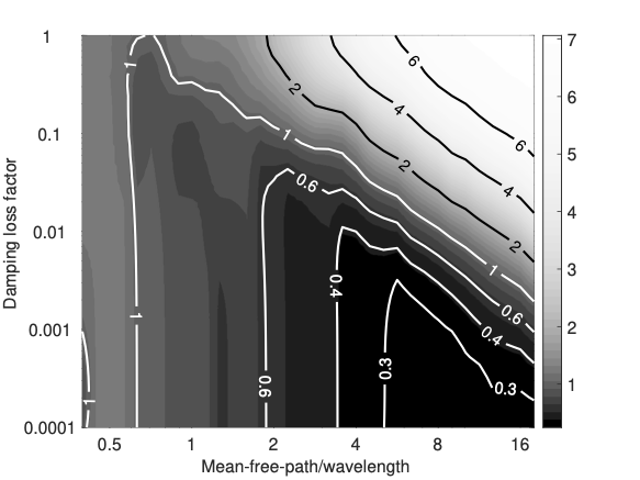
But a ray loses energy as it propagates. And for mixing to occur, the ray must be able to reflect a large number of times before disappearing. A ray of unit energy has energy \(e^{-\eta\omega t}\) after a travel of time \(t\). But the time to travel a mean-free-path \(l\), mean distance between two successive reflections, is \(t=l/c\) and the final energy is \(e^{-\eta\omega l / c}\). A weak attenuation between two reflections is equivalent to a low value of the normalized attenuation factor \(m=\eta\omega l / c\). In the following figure is shown the standard deviation of spatial fluctuations of energy in a thin plate excited in bending vibrations by a single random force. The zone where the energy is most uniformly distributed is at high frequency \(N>>1\) and low attenuation \(m << 1\).

Diffuse field map

Standard deviation of spatial fluctuations of energy in the frequency - damping plane. The zone of diffuse field map is under the isovalue line \(0.3\).

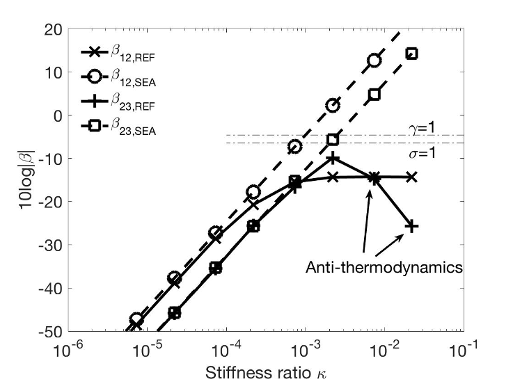
The coupling between adjacent subsystems must be weak. Imagine a bathtub filled with still water; the water's surface is perfectly flat. But when the drain is opened, the surface becomes distorted near the outlet. This is exactly the effect caused by energy leakage through coupling. The diffuse field — characterized by a homogeneous and isotropic energy distribution — becomes distorted near the coupling point. Therefore, to maintain its diffuse nature, the coupling loss must be low compared to the internal losses, which are evenly distributed across the entire surface. One must compare the coupling loss factor \(\eta_{ij}\) with the damping loss factor \(\eta_i\); the ratio \(\gamma_{ij} = \eta_{ij} / \eta_i\) must remain low.

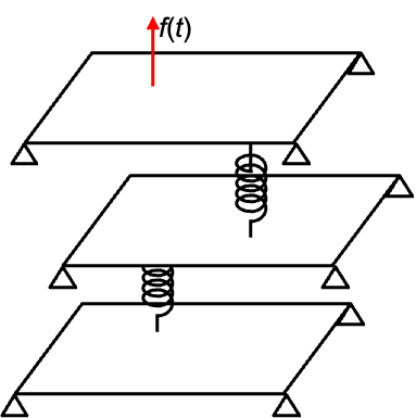
Three coupled plates

Three thin plates in bending vibration coupled by springs and excited by a random force.

Beta for three plates

Ratio \(\beta\) of exchanged power and modal energy difference versus spring stiffness.

In summary, the validity of a statistical energy analysis of vibrating mechanical systems depends on three conditions [3, 5].

  • The number of modes \(N\) in the frequency band \(\Delta\omega\) must be large in all subsystems,
    \[ N_i = n_i \Delta\omega >> 1 \]
    where \(n_i\) is the modal density.
  • The normalized attenuation factor \(m\) is low in all subsystems,
    \[ m_i = \frac{\eta_i\omega l_i}{c_i} << 1 \]
    where \(c_i\) is the group speed and \(l_i\) the mean-free-path.
  • The coupling factor \(\gamma_{ij}\) between connected subsystems is low,
    \[ \gamma_{ij} = \frac{\eta_{ij}}{\eta_i} << 1 \]
    where \(\eta_{ij}\) is the coupling loss factor and \(\eta_i\) the damping loss factor.
  1. F. Fahy, Statistical energy analyis, a critical overview. In A.J. Keane, W.G. Price, Statistical energy analysis, an overview with applications in structural dynamics, Cambridge University Press, 1996.

  2. A. Le Bot and V. Cotoni, Validity diagrams of statistical energy analysis, Journal of Sound and Vibration, vol. 329, p. 221-235, 2010.

  3. T. Lafont, N. Totaro, A. Le Bot, Review of statistical energy analysis hypotheses in vibroacoustics, Proceedings of the Royal Society A, 470, 20130515, 2013.

  4. T. Lafont, N. Totaro, A. Le Bot, Coupling strength assumption in statistical energy analysis, Proc. R. Soc. A, 473, 20160927, 2017.

  5. H. Li, N. Totaro, L. Maxit, A. Le Bot, Ergodic billiard and statistical energy analysis, Wave Motion, 87, 166-178, 2019.

  6. V. Tyrode, N. Totaro, L. Maxit, A. Le Bot, Coherent wave reflection in integrable or chaotic symmetrical acoustical billiards, Proc. R. Soc. A, 477: 2255, 2021.

Some applications

All fields of mechanical industry are concerned, aerospace, automotive, railway, energy, weapon... SEA is a powerful tool for design and optimization of structures. It allows to know energy fluxes and therefore to elaborate efficient solutions to stop the flowing of vibrational energy.

Nowadays, SEA has been adopted by almost all industries. SEA has been attractive to designers mainly because of its original insight into structural dynamics more than the efficiency of its predictive results.

Towards non-equilibrium thermodynamics...

The main difficulty encountered when applying SEA is the generally too low number of degrees of freedom in usual systems of order of few hundreds modes to be compared with Avogadro's number \(N_\text{A} = 6.02 \times 10^{23}\) in statistical physics. This has two consequences: Fluctuations about mean behaviour are very important and vibrational fields are often not diffuse.

These two shortcomings motivate an active research in laboratories up to day. The question of uncertainty in SEA is strongly connected to fluctuation theorem in statistical physics. Those of the breaking of diffuse field assumption requires the elaboration of a theory of statistical vibroacoustics beyond equilibrium analogous to the kinetic theory of gases in thermodynamics. This is what we have done with the radiative transfer equation.

Bibliography

  1. E.E. Ungar, Fundamentals of statistical energy analysis of vibrating systems, Technical report No. AFFDL-TR.66-52, 1966.

  2. R.H. Lyon, Statistical Energy Analysis of Dynamical Systems: Theory and Application, Cambridge, Massachusetts, MIT Press, 1975.

  3. R.H. Lyon and R.G. DeJong, Theory and Application of Statistical Energy Analysis, Boston, Butterworth-Heinemann, 1995.

  4. R.J.M. Craik, Sound transmission through buildings using statistical energy analysis, Boston, Gower, 1996.

  5. A.J. Keane, W.G. Price, Statistical energy analysis, an overview with applications in structural dynamics, Cambridge University Press, 1996.

  6. F.J. Fahy, W.G. Price, IUTAM symposium on statistical energy analysis, Springer, 1999.

  7. A. Le Bot, Foundation of statistical energy analysis in vibroacoustics, OUP, Oxford, 2015.